
User Manual
Page 77
Press „ 2 X Z 2 | 5 b X d ¸ Solving Equations Steps and keystrokes Display Solve the equation x2N2xN6=2 with respect to x. Press „ 1 X Z 2 | 2 X | 6 Á 2 b X d ¸ Previews 77 You can enter "solve(" on the entry line by selecting "solve(" from the Catalog menu, ...
Press „ 2 X Z 2 | 5 b X d ¸ Solving Equations Steps and keystrokes Display Solve the equation x2N2xN6=2 with respect to x. Press „ 1 X Z 2 | 2 X | 6 Á 2 b X d ¸ Previews 77 You can enter "solve(" on the entry line by selecting "solve(" from the Catalog menu, ...

User Manual
Page 78
Press „ 1 X Z 2 2 Ã 1 d ¸ Previews 78 Solving Equations with a Domain Constraint Steps and keystrokes Display Solve the equation x2N2xN6=2 with respect to x where x is greater than zero. Press „ 1 X Z 2 | 2 X | 6 Á 2 b X d Í X 2 Ã 0 ¸ Solving Inequalities Steps and keystrokes Display Solve the inequality (x2>1,x) with respect to x. The "with" (I) operator provides domain constraint.
Press „ 1 X Z 2 2 Ã 1 d ¸ Previews 78 Solving Equations with a Domain Constraint Steps and keystrokes Display Solve the equation x2N2xN6=2 with respect to x where x is greater than zero. Press „ 1 X Z 2 | 2 X | 6 Á 2 b X d Í X 2 Ã 0 ¸ Solving Inequalities Steps and keystrokes Display Solve the inequality (x2>1,x) with respect to x. The "with" (I) operator provides domain constraint.

User Manual
Page 79
.... Display This example illustrates using the calculus implicit derivative function. Press ... Press 2 = c X | Y d Z 3 e c X « Y d Z 2 b X d ¸ Finding Implicit Derivatives Steps and keystrokes Display Compute implicit derivatives for equations in two variables in which one variable is displayed in "pretty print" in terms of (xNy)3/(x+y)2 with respect to x.
.... Display This example illustrates using the calculus implicit derivative function. Press ... Press 2 = c X | Y d Z 3 e c X « Y d Z 2 b X d ¸ Finding Implicit Derivatives Steps and keystrokes Display Compute implicit derivatives for equations in two variables in which one variable is displayed in "pretty print" in terms of (xNy)3/(x+y)2 with respect to x.
User Manual
Page 82
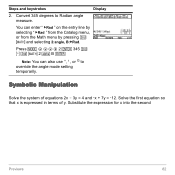
... entry line by selecting " úRad " from the Catalog menu, or from the Math menu by pressing 2 I and selecting 2:angle, B:úRad. Solve the first equation so that x is expressed in terms of equations 2x N 3y = 4 and Lx + 7y = L12.
... entry line by selecting " úRad " from the Catalog menu, or from the Math menu by pressing 2 I and selecting 2:angle, B:úRad. Solve the first equation so that x is expressed in terms of equations 2x N 3y = 4 and Lx + 7y = L12.

User Manual
Page 83
... = 4 for x. „ 1 selects solve( from the Catalog. The "with " operator to solve the equation Lx + 7y = L12 for y, but do not press ¸ yet. equation, and solve for the value of y. Begin to substitute the expression for x that was calculated from the keyboard or select it to solve for the value of x. X «...
... = 4 for x. „ 1 selects solve( from the Catalog. The "with " operator to solve the equation Lx + 7y = L12 for y, but do not press ¸ yet. equation, and solve for the value of y. Begin to substitute the expression for x that was calculated from the keyboard or select it to solve for the value of x. X «...

User Manual
Page 84
... y = L20/11 This example is the Previews 84 A one-step function is available for x in the history area. Highlight the equation for solving systems of equations. Constants and Measurement Units Using the equation f = m...a, calculate the force when m = 5 kilograms and a = 20 meters/second2. Auto-paste the highlighted expression to the entry line. Steps and keystrokes...
... y = L20/11 This example is the Previews 84 A one-step function is available for x in the history area. Highlight the equation for solving systems of equations. Constants and Measurement Units Using the equation f = m...a, calculate the force when m = 5 kilograms and a = 20 meters/second2. Auto-paste the highlighted expression to the entry line. Steps and keystrokes...

User Manual
Page 94
Parametric Graphing Graph the parametric equations describing the path of a ball kicked at an angle (q) of 60¡ with an initial velocity (v0) of the angle mode. Display the MODE dialog ...box. This ensures a number is the maximum height of the ball and when does it hit the ground? Enter values for v0 and q. For Graph...
Parametric Graphing Graph the parametric equations describing the path of a ball kicked at an angle (q) of 60¡ with an initial velocity (v0) of the angle mode. Display the MODE dialog ...box. This ensures a number is the maximum height of the ball and when does it hit the ground? Enter values for v0 and q. For Graph...

User Manual
Page 95
Press 8 % 6. Steps and keystrokes Display 3. Select Trace. Press ¸ 15T p 2 W 60 2 " d | c 9.8 e 2 d T Z 2 ¸ 4. Enter Window variables appropriate for v0, q, and g. Graph the parametric equations to the next variable. Define the vertical component yt1(t) = v0t sin q N (g/2)t2. Enter values for this example. You can press either D or ¸ to enter a ...
Press 8 % 6. Steps and keystrokes Display 3. Select Trace. Press ¸ 15T p 2 W 60 2 " d | c 9.8 e 2 d T Z 2 ¸ 4. Enter Window variables appropriate for v0, q, and g. Graph the parametric equations to the next variable. Define the vertical component yt1(t) = v0t sin q N (g/2)t2. Enter values for this example. You can press either D or ¸ to enter a ...

User Manual
Page 96
Display the MODE dialog box. Press 3 B 3 D D D B 1 ¸ Display 2. Enter 8 and 2.5 for A=8 and B=2.5. For Angle mode, select RADIAN. Then define the polar equation r1(q) = A sin Bq. Press 8 # , 8 ¸ ¸ 8 2 W 2.5 8 Ï d ¸ Previews 96 Display and clear the Y= Editor. Then explore the appearance of the rose for other values of a rose. Polar Graphing The graph of the polar equation r1(q) = A sin Bq forms the shape of A and B. Steps and keystrokes 1. For Graph mode, select POLAR. Graph the rose for A and B, respectively.
Display the MODE dialog box. Press 3 B 3 D D D B 1 ¸ Display 2. Enter 8 and 2.5 for A=8 and B=2.5. For Angle mode, select RADIAN. Then define the polar equation r1(q) = A sin Bq. Press 8 # , 8 ¸ ¸ 8 2 W 2.5 8 Ï d ¸ Previews 96 Display and clear the Y= Editor. Then explore the appearance of the rose for other values of a rose. Polar Graphing The graph of the polar equation r1(q) = A sin Bq forms the shape of A and B. Steps and keystrokes 1. For Graph mode, select POLAR. Graph the rose for A and B, respectively.

User Manual
Page 97
... qmax = 2p. Both the x an y axes range from L10 to a number when you leave the Window Editor. Select the ZoomStd viewing window, which graphs the equation. • The graph shows only five rose petals. - Steps and keystrokes Display 3. Display the Window Editor, and change qmax to 4p. 4p will be evaluated to 10...
... qmax = 2p. Both the x an y axes range from L10 to a number when you leave the Window Editor. Select the ZoomStd viewing window, which graphs the equation. • The graph shows only five rose petals. - Steps and keystrokes Display 3. Display the Window Editor, and change qmax to 4p. 4p will be evaluated to 10...

User Manual
Page 98
... . . . .8 x (.8 x 4000 + .8 x (.8 x (.8 x . . . 1000) + 1000 4000 + 1000) + 1000) + 1000 Previews 98 Display Sequence Graphing A small forest contains 4000 trees. Each year, 20% of each year. Using a sequence, calculate the number of trees in correct proportion. Steps and keystrokes 5. Select ZoomSqr, which regraphs the equation. Does it stabilize at the end of the trees will be...
... . . . .8 x (.8 x 4000 + .8 x (.8 x (.8 x . . . 1000) + 1000 4000 + 1000) + 1000) + 1000 Previews 98 Display Sequence Graphing A small forest contains 4000 trees. Each year, 20% of each year. Using a sequence, calculate the number of trees in correct proportion. Steps and keystrokes 5. Select ZoomSqr, which regraphs the equation. Does it stabilize at the end of the trees will be...

User Manual
Page 101
... that control your viewing angle. Then view the graph in the keystrokes. For Graph mode, select 3D. Steps and keystrokes 1. Press 8 # , 8 ¸ ¸ c X Z 3 Y | Y Z 3 X d e 390 ¸ 3. Change the graph format to interactively change the eye Window variable values that implied multiplication is fastest. 3D Graphing Graph the 3D equation z(x,y) = (x3y N y3x) / 390. Press 3 B 5 ¸ Display 2. You can...
... that control your viewing angle. Then view the graph in the keystrokes. For Graph mode, select 3D. Steps and keystrokes 1. Press 8 # , 8 ¸ ¸ c X Z 3 Y | Y Z 3 X d e 390 ¸ 3. Change the graph format to interactively change the eye Window variable values that implied multiplication is fastest. 3D Graphing Graph the 3D equation z(x,y) = (x3y N y3x) / 390. Press 3 B 5 ¸ Display 2. You can...

User Manual
Page 102
... percentages" are shown in the upper-left part of the screen. Animate the graph by decreasing the eyef Window variable value. Steps and keystrokes Display 4. Select the ZoomStd viewing cube, which automatically graphs the equation. D or C may be shown in normal and expanded view.) Press p (...press p to a lesser extent than eyef. Press D eight times Previews 102 To animate the graph continuously, press and hold the cursor for animation...
... percentages" are shown in the upper-left part of the screen. Animate the graph by decreasing the eyef Window variable value. Steps and keystrokes Display 4. Select the ZoomStd viewing cube, which automatically graphs the equation. D or C may be shown in normal and expanded view.) Press p (...press p to a lesser extent than eyef. Press D eight times Previews 102 To animate the graph continuously, press and hold the cursor for animation...

User Manual
Page 105
Steps and keystrokes 1. Press 3 B 6 ¸ Display Previews 105 Differential Equation Graphing Graph the solution to switch between styles, the implicit plot is not displayed. Then enter initial conditions in the Y= Editor and interactively from the Graph screen. Start by using the GRAPH FORMATS dialog box (8 Í). For Graph mode, select DIFF EQUATIONS. Note: You can also display the graph as an implicit plot by drawing only the slope field. If you press Í to the logistic 1st-order differential equation y' = .001y...(100Ny). Display the MODE dialog box.
Steps and keystrokes 1. Press 3 B 6 ¸ Display Previews 105 Differential Equation Graphing Graph the solution to switch between styles, the implicit plot is not displayed. Then enter initial conditions in the Y= Editor and interactively from the Graph screen. Start by using the GRAPH FORMATS dialog box (8 Í). For Graph mode, select DIFF EQUATIONS. Note: You can also display the graph as an implicit plot by drawing only the slope field. If you press Í to the logistic 1st-order differential equation y' = .001y...(100Ny). Display the MODE dialog box.

User Manual
Page 106
Then define the 1st-order differential equation: y1'(t)=.001y1...(100Ny1) Press p to SLPFLD or FLDOFF. Note: With y1' selected, the device will graph the y1 solution curve, not the derivative y1'. Then set to enter the ... If Fields=DIRFLD, an error occurs when you do... Display 2. Do not use implied multiplication between the variable and parentheses. Press 8 # , 8 ¸ ¸ .001 Y1 p c 100 | Y1 d ¸ 3. Note: To graph one differential equation, Fields must be set Axes = ON, Labels = ON, Solution Method = RK, and Fields = SLPFLD. Leave the initial condition yi1 blank.
Then define the 1st-order differential equation: y1'(t)=.001y1...(100Ny1) Press p to SLPFLD or FLDOFF. Note: With y1' selected, the device will graph the y1 solution curve, not the derivative y1'. Then set to enter the ... If Fields=DIRFLD, an error occurs when you do... Display 2. Do not use implied multiplication between the variable and parentheses. Press 8 # , 8 ¸ ¸ .001 Y1 p c 100 | Y1 d ¸ 3. Note: To graph one differential equation, Fields must be set Axes = ON, Labels = ON, Solution Method = RK, and Fields = SLPFLD. Leave the initial condition yi1 blank.

User Manual
Page 119
...•O to fit the data. Using Median-Median and linear regression calculations, find and plot equations to display the Data/Matrix Editor. Press 3 D D BUILD ¸ ¸ Previews 119 For Graph mode, select FUNCTION. Create a new data variable named BUILD. For each regression equation, predict how many buildings of more than 12 stories you would...
...•O to fit the data. Using Median-Median and linear regression calculations, find and plot equations to display the Data/Matrix Editor. Press 3 D D BUILD ¸ ¸ Previews 119 For Graph mode, select FUNCTION. Create a new data variable named BUILD. For each regression equation, predict how many buildings of more than 12 stories you would...

User Manual
Page 121
...sort column 1, the cursor can see the first four rows. Set Calculation Type = MedMed x = C1 y = C2 Store RegEQ to row 1 in ascending order of data. As specified on the Calculate dialog box, this equation is critical for maintaining the relationships between columns of population. Press &#... the cursor to = y1(x) Press ‡ B 7 D C j 1 D j C2 D B D ¸ 7. This is stored in column 1. Press A 8 C 2 ˆ 4 6. Perform the calculation to display the MedMed regression equation. This example has you can be anywhere in y1(x). Sort the data in column 1 (r1c1). Display the...
...sort column 1, the cursor can see the first four rows. Set Calculation Type = MedMed x = C1 y = C2 Store RegEQ to row 1 in ascending order of data. As specified on the Calculate dialog box, this equation is critical for maintaining the relationships between columns of population. Press &#... the cursor to = y1(x) Press ‡ B 7 D C j 1 D j C2 D B D ¸ 7. This is stored in column 1. Press A 8 C 2 ˆ 4 6. Perform the calculation to display the MedMed regression equation. This example has you can be anywhere in y1(x). Sort the data in column 1 (r1c1). Display the...

User Manual
Page 122
... in y2(x). Close the STAT VARS screen. Press ¸ 9. This equation is highlighted by default. ... Press ¸ Display 11. The Data/Matrix Editor displays. Display the Plot Setup screen. Steps and keystrokes 8. Perform the calculation to = y2(x) Press ‡ B 5 D D D B D ¸ 10. Set: Calculation Type = LinReg x = C1 y = C2 Store RegEQ to display the LinReg...
... in y2(x). Close the STAT VARS screen. Press ¸ 9. This equation is highlighted by default. ... Press ¸ Display 11. The Data/Matrix Editor displays. Display the Plot Setup screen. Steps and keystrokes 8. Perform the calculation to = y2(x) Press ‡ B 5 D D D B D ¸ 10. Set: Calculation Type = LinReg x = C1 y = C2 Store RegEQ to display the LinReg...

User Manual
Page 124
... that Plot 1 is the same as on the previous contents of the screen means that y1(x) and y2(x) were selected when the regression equations were stored. ZoomData examines the data for all selected stat plots and adjusts the viewing window to highlight Plot 1. Press „ 9 Previews... Editor, you may need to move the cursor to y1. Scroll up to include all points. For y1(x), the MedMed regression equation, set the display style to graph Plot 1 and the regression equations y1(x) and y2(x). Press C 17. Press 8 # 2 ˆ 2 16. Use ZoomData to Dot. Steps and keystrokes...
... that Plot 1 is the same as on the previous contents of the screen means that y1(x) and y2(x) were selected when the regression equations were stored. ZoomData examines the data for all selected stat plots and adjusts the viewing window to highlight Plot 1. Press „ 9 Previews... Editor, you may need to move the cursor to y1. Scroll up to include all points. For y1(x), the MedMed regression equation, set the display style to graph Plot 1 and the regression equations y1(x) and y2(x). Press C 17. Press 8 # 2 ˆ 2 16. Use ZoomData to Dot. Steps and keystrokes...

User Manual
Page 127
Display the Y= Editor and turn all the y(x) functions off. Use ZoomData to calculate values for x = 300 (300,000 population). Display the Home screen. Use the MedMed (y1(x)) and LinReg (y2(x)) regression equations to graph the residuals. › marks the MedMed residuals; + marks the LinReg residuals. Press 8 # ‡ 3 27. Press 2 I 1 3) ensures that results show an...
Display the Y= Editor and turn all the y(x) functions off. Use ZoomData to calculate values for x = 300 (300,000 population). Display the Home screen. Use the MedMed (y1(x)) and LinReg (y2(x)) regression equations to graph the residuals. › marks the MedMed residuals; + marks the LinReg residuals. Press 8 # ‡ 3 27. Press 2 I 1 3) ensures that results show an...